Detecting influential observations using psignifit
When fitting psychometric functions using psignifit, we usually look for a suitable descriptive model of our recorded data. Thus, it is of interest to make sure that the psychometric function actually captures the structure of the whole data set and not of just a single data point. We call a data point that heavily influences the fitted model an influential observation. [Wichmann_and_Hill_2001a] suggest to detect influential observations using a sort of jackknife procedure. This strategy is at the heart a classical frequentist approach to the detection of influential observations. We will first explain how psignifit implements this procedure and then show how to use a similar procedure to determine influential observations in Bayesian terms.
If you haven’t generated the example dataset named “data_single_sessions”, you can find it here.
Influential observations in bootstrapped data
The procedure to detect influential observations that was suggested by [Wichmann_and_Hill_2001a] starts with the regular bootstrap confidence intervals as obtained by the bootstrap procedure. We apply this procedure to the example from the tutorial: If you haven’t created the Bootstrap Inference Object and done the sampling, do:
>>> B_single_sessions = psi.BootstrapInference ( data_single_sessions, priors=("unconstrained","unconstrained","Beta(2,20)"), sample=True )
>>> B_single_sessions.infl.round(2)
array([ 0.34,  0.02,  0.19,  0.13,  0.15,  0.21,  0.43,  0.19,  0.86,
        0.15,  0.06,  0.4 ,  0.02,  0.13,  0.15])
What do these numbers tell us? Obviously, the last block has a relatively high “influence” here, while the second to last has a lower “influence”.
In order to detect influential observations, [Wichmann_and_Hill_2001a] suggest to generate a number of
new data sets  by leaving out the
  -th data block. We fit a psychometric function to each of these
new data sets. If the psychometric function fitted to data set
  is significantly different from the psychometric
function fitted to the whole data set, block
  is considered influential.
Thus, for a parameter
  , we define for dataset
  the following quantity
If  , where
  is the complete dataset

else

 is simply the distance between the fit to the whole dataset and the reduced dataset
  , where the distance
has been scaled such that a value of
  indicates that the respective parameter in the reduced dataset
lies precisely on the border of the confidence interval for parameter i in the full data set.
The influence of a data point is then simply defined as the maximum of the
  over all parameters i.
Thus, the relatively high influence of 0.95 for the last block is still not really serious. All parameter
estimates for reduced data sets are still perfectly within the confidence limits of the full data set.
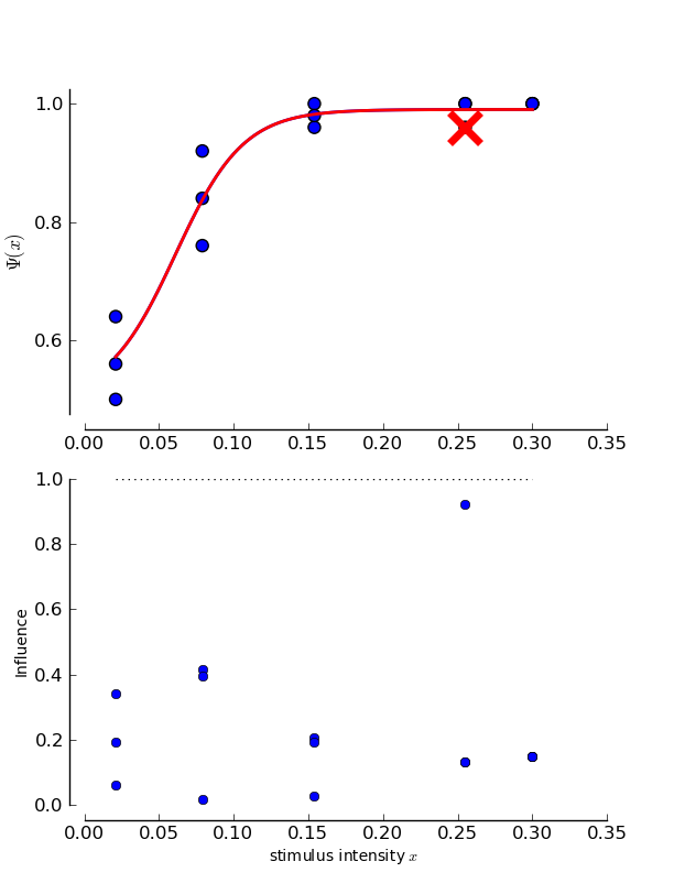
Typcially, we want to visualize the influence of the datapoints to get a quick idea of the influences of the individual data points. To do so, we can use the plotInfluential() method
>>> psi.plotInfluential(B_single_sessions)

This will give us two plots. The upper plot simply redraws the psychometric function. In addition to the psychometric function, the data points are shown. To indicate the influence of the strongest data point, this point is marked by a red x and the fit to the reduced data set is also drawn in red. We can observe here the same things as we noted before: The last point is marked as the most influential and if it is excluded from the fit, the psychometric function is not seriously altered.
The plot at the bottom displays an overview over the influence of all data points. In addition to the influence values, there is a dotted line to mark the point above which psychometric functions fitted to the reduced data set would significantly differ from the fit to the whole data set.
We can note here that it is reasonable that actually the only serious difference between the fit to the whole data set and
the fit to the reduced dataset might originate from a difference in the lapse rate. (It is as you can see if you calculate
the  manually). In many cases, the lapse rate is considered a nuissance parameter. Usually what we want to know is more
like “is the whole inference influenced by this one data point”. It is difficult to derive a riguorous definition for this
kind of influence in a frequentist setting, even in a relatively data driven frequentist setting such as the employed
bootstrap procedure. However, in a Bayesian setting such an influence measure is readily available.
Influential observations in Bayesian Inference
Instead of performing inference on specific values of parameters, i.e. on point estimates, Bayesian inference treats the whole probability distribution of the parameters after observing the data. This is the reason, why a Bayesian setting is well adapted to the problem of estimating the influence of a single data point on the whole inference. We measure the influence of data block k by comparing the posterior distribution given the whole data set to the posterior distribution of the data set d_k. A suitable measure for the differences between two distributions is the Kullbach-Leibler divergence. High Kullbach-Leibler divergences indicate large differences between the two distributions and thus a strong influence of the respective data block, while low Kullbach-Leibler divergences indicate low influence of the respective data block. Kullbach-Leibler divergence is an information theoretic measure. The exact interpretation of Kullbach-Leibler divergence would be in terms of optimal coding lengths and can be found in introductury texts like [Bishop_2006].
The influence of data blocks is calculated in terms of Kullbach-Leibler divergence for BayesInference objects.
>>> mcmc = BayesInference ( data, priors=('Gauss(0,5)', 'Gamma(1,3)', 'Beta(2,30)') )
>>> mcmc.infl.round(2)
array([ 0.42,  0.46,  0.12,  0.15,  0.33,  0.05])
We can see here, that the influence of the last data block is rather minor in terms of the changes to the whole distribution. Thus, Kullbach-Leibler divergence does not necessary give the same results as the bootstrap/jackknife based procedure described above and suggested by [Wichmann_and_Hill_2001a].
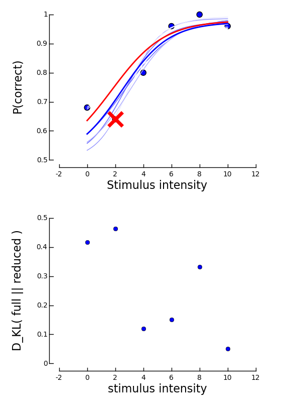
We can visualize the data influence again using
>>> plotInfluential(mcmc)

The plot highly resembles the plot obtained for the bootstrap case. At the top, the fitted psychometric function is plotted along with the data. Again, the most influential data point is marked by a red x and the psychometric function associated with the data set in which this point was excluded is drawn in red. The get an idea of other typical posterior psychometric functions, 20 sample psychometric functions are drawn in this plot in shades of blue. We can immediately see, that the red curve is very similar to the blue different blue shaded curves.
The bottom plot displays the Kullbach-Leibler divergences for all blocks. We can observe that the strongest influence on the posterior distribution is from the block with stimulus intensity 2. Note, however, that a Kullbach-Leibler divergence of 0.46 is still very low.
